In an earlier blog we examined the decumulation performance of CDC schemes under deterministic investment returns and inflation.

This blog considers the excessive volatility and the wildness of outcome introduced by random annual market returns, using stochastic simulation of a particular contribution history. It draws attention to the weaknesses of some CDC business models and problems arising from the CDC-enabling legislation and proposed code of practice.

The Set-Up

We consider contributions of 15% of salary, with salary rising at 2% pa from age 25 until retirement at age 65, with an initial starting salary of £30,000. We use the same survival table as in the earlier blog (it is gender neutral extending to age 105 and implies a life expectation of 88.5 years at age 65).

We conducted a 5,000 iteration Monte Carlo simulation of the achieved performance. In order to achieve, on average, the 5% deterministic (or geometric) return rate indicated in the earlier blog, we sample randomly from a Normal distribution of returns (µ =6.125%, σ = 15%).

The first point to note is that there is significant extreme variation in the outcome of the accumulation phase. Figure 1 shows the distribution of accumulated values of the pension pot at age 65. Given the limitations of Excel’s graphics, this is a random sample of 100 of the simulations.

Figure 1: Pot Values at Age 65

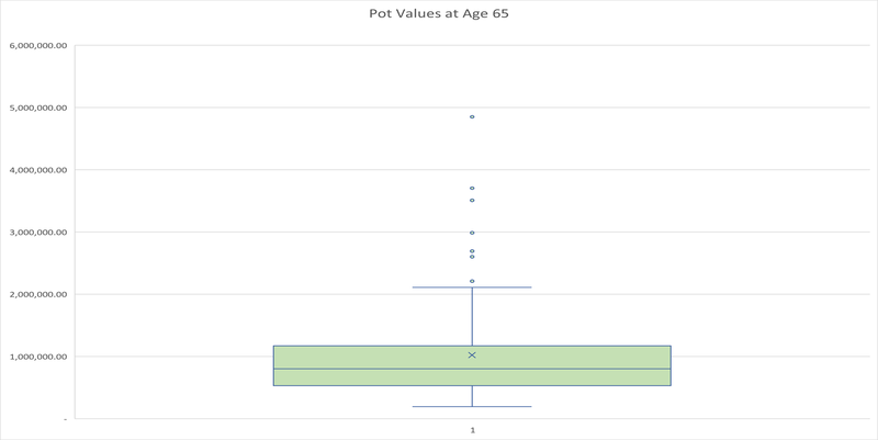
The pot value varies wildly, from as little as £195,819.90 to as much as £4,850,714.41. The deterministic value of the pot at retirement is £948,703.48. The mean and median statistics for the displayed sample are £981,647.97 and £809,582.86 respectively.

We should add an important caveat to interpretation of this distribution; this is the range of possible outcomes but that is not a predictor of the distribution of actual outcomes expected when many CDC schemes exist. When there are numerous CDC schemes, we may expect many to adopt similar and possibly even identical investment strategies, including the use of indexed portfolios, which will limit the range of outcomes. There is no ergodic relationship between these.

The level annuities associated with these pots, with perfect foresight of the stochastic returns achieved in the retirement period, are shown in the second box and whiskers chart in Figure 2 below. As is to be expected these also vary wildly, from a low of £9,457.87 pa to as much as £491,795.32. We have not taken account of any taxation effects, such as lifetime allowances as doing so would mask the variability and are an artefact of current policy rather than a permanent limiting factor. It is also worth noting that the worst pension is not associated with the minimum pot value, but rather another iteration, which had a pot value of £209,607.95; the £195,819.90 produced a level pension of £ 26,613.25, which clearly illustrates randomness at work.

Figure 2: Level Pensions with Perfect Foresight (for sample of Figure 1)

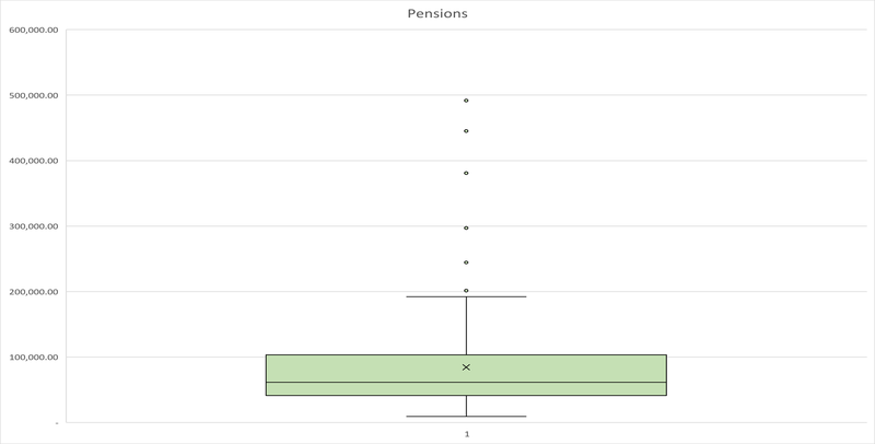
Figure 3 shows the relation between the perfect foresight level annuity and the pot value at retirement. The blue circle marker is the deterministic pot and annuity couplet.

Figure 3: Pot and Level Annuity Values

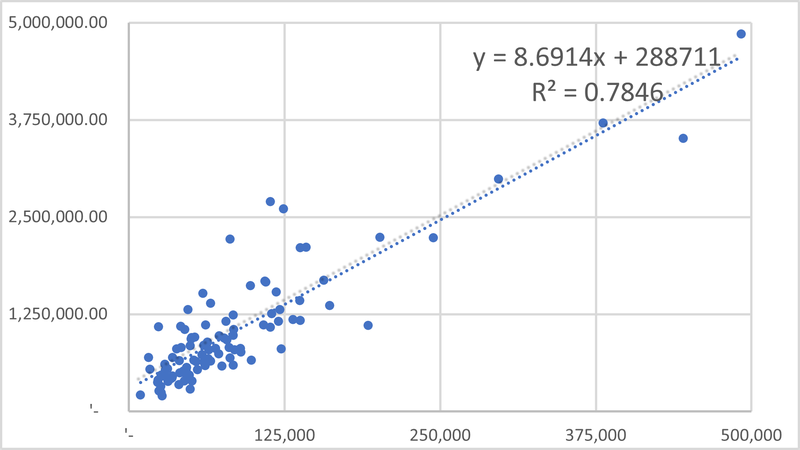
The linear regression above shows that there is a strong but not perfect relation between pot size and achievable annuity. Though not immediately obvious from this diagram, the variability of the retirement income (albeit measured in this perfect foresight manner) is considerably higher than the variability of pot outcomes at retirement.

Of course, we do not possess perfect foresight, which limits the inferences that can be made.

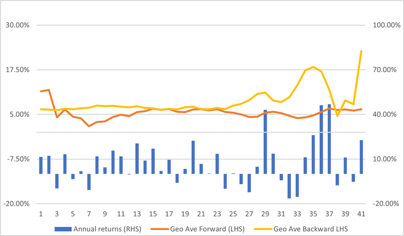
We will consider, for pedagogic purposes, a single randomly chosen iteration from the Monte Carlo collection. The annual returns for this are shown graphically in Figure 4 below, which also shows the geometric values of the sequence. Firstly, in the usual manner, moving forwards in time – the experienced geometric return, and secondly, moving backwards in time from the final return achieved – this is the ‘to-be’ experienced geometric return. We will return to this latter metric later. Table 1 reports the descriptive statistics of the post-retirement returns sequence.

Table 1: Descriptive Statistics - Post-retirement Returns Sequence

Median 6.82%

Mean 7.46%

Geo Mean 6.45%

St Dev 15.31%

Min -16.41%

Max 46.88%

The sample sequence has a pot value at retirement of £654,761.91. This particular sample underperformed the base case in accumulation but outperforms in decumulation, and in overall performance (6.45% versus 5%). Inspection of the geometric returns in Figure 4, shows that in decumulation, the chosen sequence underperforms the 5% deterministic rate in its early evolution but outperforms in the latter stages.

Figure 4: Sample returns series - Annual and Geometric Average Investment Returns

The conversion of the pension pot to a retirement income may be done in two distinct manners. The first approach is where a lifetime pension, which may be level or indexed, can be set at retirement (effectively an annuity) and any surpluses or deficits arising from investment performance in a year are then paid as bonuses to the pensioner in that year, or in the case of deficits, are demanded from him or her. The second approach is to reset the pension rate in each year, such that the scheme satisfies the statutory annual balance requirement directly.

Several reviewers suggested that the first, the basic pension and bonus structure would be simpler and therefore preferable to the second option. Unfortunately, this basic plus structure is most unlikely to produce the stability of retirement income desired. In Figure 5, we show the basic indexed pension which may be created from the retirement pot of £654,761.91, together with the annual bonus/malus.

In arriving at these annuity values, and the indexed values reported later, we have continued to assume a 5% rate of investment return for remaining future periods. In fact, given the underperformance of the returns to the contributions made in the accumulation period, there would have been pressure to use a lower assumed rate. In the post retirement period this would have been compounded by the fact that the achieved post-retirement geometric return to age 72 is just 1.69%.

Figure 5: Pension & Bonus

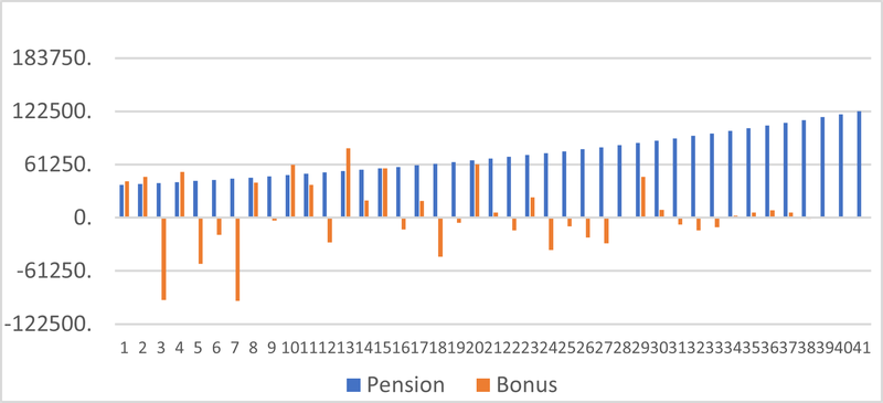
The problems arise from the fact that on twenty occasions, the pensioner would be called upon to contribute i.e., pay money into the scheme. In sixteen of these, the amount exceeds HMRC’s annual limit of £4,000 on contributions to a scheme once the pension is in payment. Three events would also, on their own, exceed the annual allowance.

Figure 6 shows the total income arising in a year, which is the sum of pension and bonuses. We see that there are three years in which the pensioner would on balance be required to contribute more than their pension income and that two of these are substantial – in excess of £50,000. The base plus bonus approach is simply excessively volatile. The bonus element has a mean value of £3,038.61, but with volatility of £38,169.20.

Figure 6: Total Pension and Components

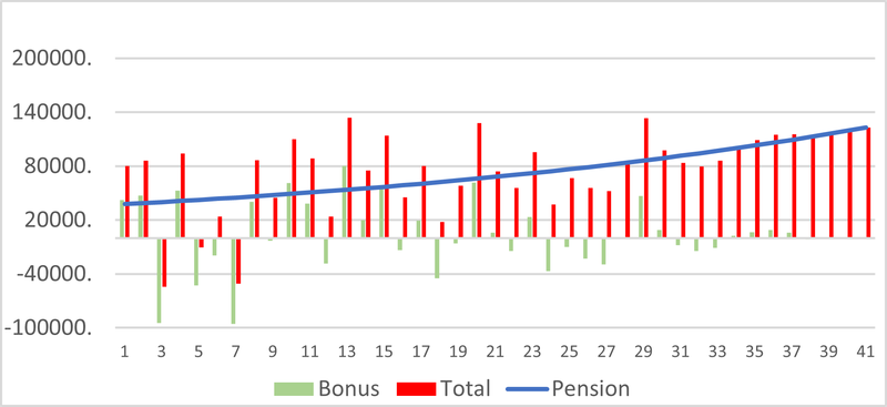
Simply put, we do not believe that a pensioner would find this instability in income to be acceptable.

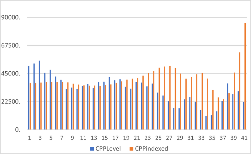
As the essence of CDC schemes is the ability to modify the pension in payment, we next examine the variability from year to year of an annually repriced level pension for this single iteration – Figure 7 below.

Figure 7: Level Annuity Variation and Constant Purchasing Power Equivalent

We show the level annuity value of the residual value of the pot after accrual of that year’s random return, after payment of the pension annuity value. In each year, the level annuity value would persist for the residual term of the annuity but is supplanted in each year by the (new) level annuity rate, which maintains asset and liability balance. The pension varies from year-to-year, reflecting the experienced investment performance.

The statutory requirement to balance assets and liabilities annually leads to this variation. The descriptive statistics of the (quasi) level pension are shown in Table 2. This variability is substantial; there are proportional cuts of 26%, 27% and 28% in this iteration. There are twenty years in which cuts to the pension are needed and there are sixteen years in which the pension payable is below the initial level. This variability could easily give rise to a lack of confidence and trust on the part of scheme members.

Figure 7 also shows the purchasing power of the pension. The rate of inflation is a constant 3% pa. As is to be expected it shows a steady decline over time.

Table 2: Descriptive Statistics of (Quasi) Level Pension

Median 56,325.79

Mean 57,238.81

St. Dev 16,228.19

Min 29,453.43

Max 110,925.96

It should also be added that the extreme variation of the final few years is related to properties of the return sequence and to the inherent instability of the survival probabilities at ages beyond 100, including the fact that the age 105 value is a truncation of all lives that survive beyond that. We will demonstrate this later, as Figure 9, in the case of indexed pensions where the instability is more pronounced.

The indexed pension also shows variability from year-to-year, speaking loosely, in a similar manner to the level pension. Figure 8 shows the progression of the pension annuity value, from the same pot at retirement as previously. It also shows the progression of a comparable deterministic (µ =25%, σ = 3%) pension annuity from that initial pot. Note that the scale in Figure 8 is logarithmic.

Figure 8: Indexed Pension and (5%, 3%) deterministic Comparator

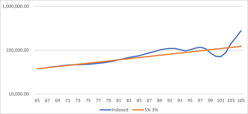
There are just six years in which pensions are cut, and though the largest annual decline is only 20%, there is a four-year sequence which results in a 40% decline in the pension. The subsequent two years of 40% plus returns ‘save the day’ and together with the longevity or survival effects, already mentioned, in the later years of the iteration lead to exponential growth. In part, this is because, to maintain consistency with the earlier level annuity, we assume continuation of this latest level of indexation.

The relation between the revalued indexed pension and (backward geometric) investment returns is shown in Figure 9, the returns are the source of much of the later stage instability evident in both level and indexed pensions. The three year-return sequence when begins seven years from maturity multiplies the investment returns by a factor of 2.7. The likelihood of observing two such 40+% returns (or higher) is very small, just 0.0012%.

While the pension payable to surviving scheme members increases exponentially, it should not be forgotten that the number surviving is very small. The absolute cost to the scheme of these pensions is small and declining over the final few years. There is here the potential for a mis-selling case since illustrations showing just the pension to be payable do not take account of the member’s likelihood of surviving to receive those very large pensions.

Figure 9: Revalued Indexed Pension and Investment Returns

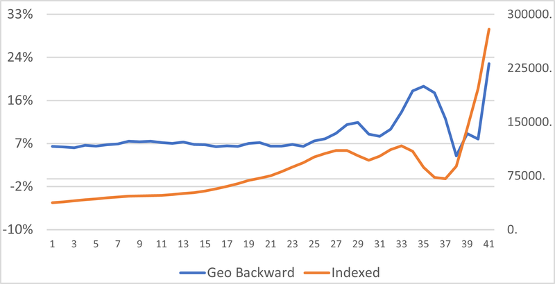
Figure 10 shows the level of indexation applied from year-to-year and a smoothed version of this: the year-to-date cumulative average indexation. This is far smoother than the annual variation; that is 15 times as volatile as the cumulative indexation – its largest decline is 0.78% index points. The descriptive statistics for the indexed series are shown at Table 3.

Table 3: Descriptive Statistics for the Indexed Series

Median 71,769

Mean 81,605

St. Dev 45,877

Min 37,696

Max 279,252

Figure 10: Annual And Cumulative Indexation Rates

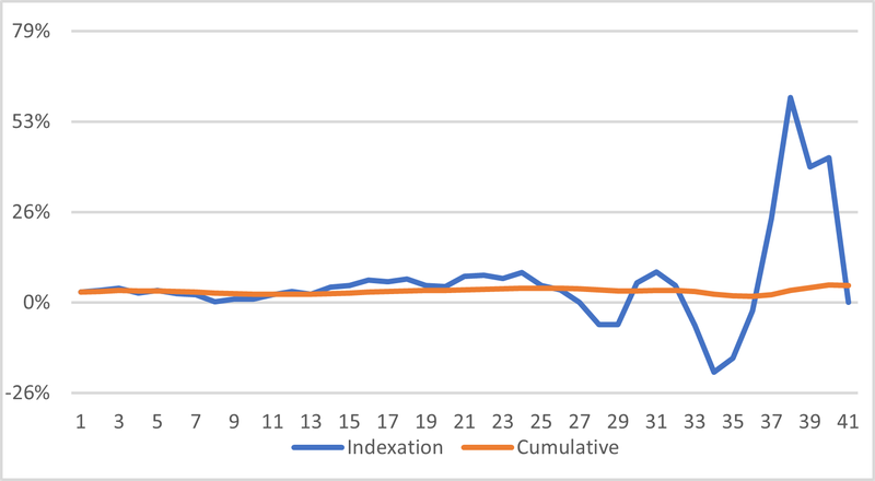
Unfortunately, such smoothing would not be permitted under the CDC Regulations and proposed CDC Code.

Next, we show in Figure 11, the level annuity and indexed annuity evolutions.

Figure 11: Level and Indexed Pensions

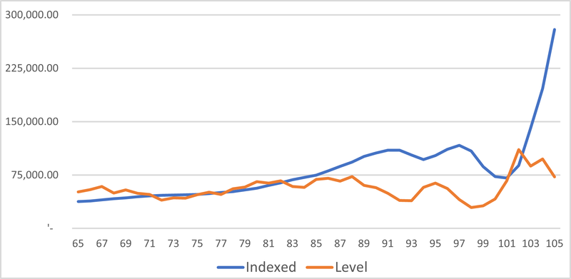
Finally, we show, as Figure 12, the constant purchasing power of the level and indexed pensions, the real pensions. Both series are adjusted using the assumption of a constant rate of inflation of 3% pa. It is only in the 90th year that the total receipts from an indexed pension exceed those from a level arrangement. Of course, as was shown in the earlier blog, the total pension received over the member’s lifetime in retirement is greater for the indexed pension than the level, reflecting the slower rate of depletion and higher investment returns this facilitates.

Figure 12: Level and Indexed Pensions in Real or Constant Purchasing Power terms

Some have promoted indexed CDC as being superior to level CDC in the sense that a member will be less likely to experience cuts to their nominal pension. The idea here is that the indexation term serves as a risk buffer. It is a very substantial buffer – the level pension is 36% higher than the indexed at inception. However, as we have seen earlier, even that may not be sufficient to ensure no cuts.

Some have suggested that indexation may be used as a risk buffer by variation of not both the current and future level as has been the case in this blog, but by variation only of the future indexation. In fact, risk management conducted in this manner need not be limited to indexed pensions. It is perfectly possible for a level scheme to announce cuts scheduled to occur in the future. This is redolent of the Augustinian prayer: "Oh Lord, make me chaste but not yet". Its potential for time inconsistency and ensuing financial crisis are substantial. If trustees can maintain scheme balance by varying future indexation without cost today, they can be expected to avail themselves of this to excess.

Final Thoughts

The purpose of this short blog is to highlight the impacts that the regulations and proposed CDC Code will have on design structures and outcomes, using a more realistic stochastic approach to modelling than the stylized deterministic version that we used in the previous blog. What is clear, is that the short-term prescriptions within the CDC Code and Regulations essentially remove all the benefits of CDC in a world of stochastic returns. While many would assume that the significant variability that we see is due to “riskier investments”, it is actually the constant short-term tinkering and micro-managing of the scheme induced by regulation that induces such variable outcomes. As with many other aspects of pension regulation, it is often the regulation itself that is the problem and not the underlying structure of benefits.